Engage NY Eureka Math Algebra 1 Module 2 Lesson 16 Answer Key
Eureka Math Algebra 1 Module 2 Lesson 16 Example Answer Key
Example 1.
Calculating Residuals
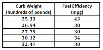
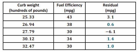
The curb weight of a car is the weight of the car without luggage or passengers. The table below shows the curb weights (in hundreds of pounds) and fuel efficiencies (in miles per gallon) of five compact cars.
Using a calculator, the least squares line for this data set was found to have the equation:
y=78.62-1.5290x,
where x is the curb weight (in hundreds of pounds), and y is the predicted fuel efficiency (in miles per gallon).
The scatter plot of this data set is shown below, and the least squares line is shown on the graph.
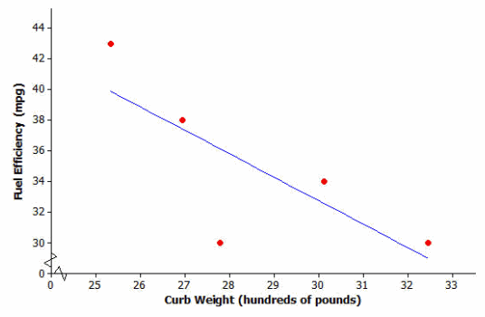
You will calculate the residuals for the five points in the scatter plot. Before calculating the residuals, look at the scatter plot.
Example 2.
Making a Residual Plot to Evaluate a Line
It is often useful to make a graph of the residuals, called a residual plot. You will make the residual plot for the compact car data set.
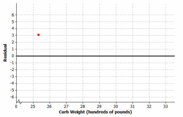
Plot the original x-variable (curb weight in this case) on the horizontal axis and the residuals on the vertical axis. For this example, you need to draw a horizontal axis that goes from 25 to 32 and a vertical axis with a scale that includes the values of the residuals that you calculated. Next, plot the point for the first car. The curb weight of the first car is 25.33 hundred pounds and the residual is 3.1 mpg. Plot the point (25.33,3.1).
The axes and this first point are shown below.
Eureka Math Algebra 1 Module 2 Lesson 16 Exercise Answer Key
Exercises 1–2
Exercise 1.
Will the residual for the car whose curb weight is 25.33 hundred pounds be positive or negative? Roughly what is the value of the residual for this point?
Answer:
Positive residual of 3 mpg; the actual value is approximately 3 units above the line.
Exercise 2.
Will the residual for the car whose curb weight is 27.79 hundred pounds be positive or negative? Roughly what is the value of the residual for this point?
Answer:
Negative residual of -6 mpg; the actual value is 6 units below the line.
Now confirm the estimated residuals by calculating the exact residuals using the least squares line as shown in the text.
The residuals for both of these curb weights are calculated as follows:
Substitute x=25.33 into the equation of the least squares line to find the predicted fuel efficiency.
y=78.62-1.5290(25.33)
=39.9
Now calculate the residual.
residual = actual y-value – predicted y-value
=43 mpg-39.9 mpg
=3.1 mpg
Substitute x=27.79 into the equation of the least squares line to find the predicted fuel efficiency.
y=78.62-1.5290(27.79)
=36.1
Now calculate the residual.
residual = actual y-value – predicted y-value
=30 mpg-36.1 mpg
=-6.1 mpg
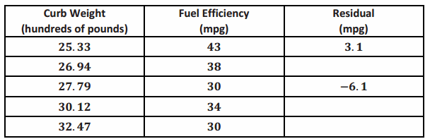
These two residuals have been written in the table below.
Exercises 3–4
Continue to think about the car weights and fuel efficiencies from Example 1.
Exercise 3.
Calculate the remaining three residuals, and write them in the table.
Answer:
The residuals are shown in the table below.
Exercise 4.
Suppose that a car has a curb weight of 31 hundred pounds.
a. What does the least squares line predict for the fuel efficiency of this car?
Answer:
y=78.62-1.5290(31)=31.2
The predicted fuel efficiency is 31.2 mpg.
b. Would you be surprised if the actual fuel efficiency of this car was 29 miles per gallon? Explain your answer.
Answer:
No. The residual for this point would be 29 mpg-31.2 mpg, or -2.2 mpg. This is within the range of the residuals for the table above.
Exercises 5–6
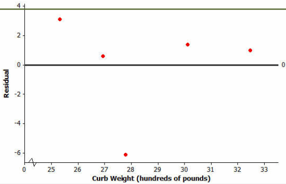
Plot the other four residuals in the residual plot started in Example 3.
Answer:
The completed residual plot is shown below.
Exercise 6.
How does the pattern of the points in the residual plot relate to the pattern in the original scatter plot? Looking at the original scatter plot, could you have known what the pattern in the residual plot would be?
Answer:
The first point in the scatter plot is quite a long way above the least squares line (compared to the distances above or below the line of most of the other points), so it has a relatively large positive residual. The second point is a relatively small distance above the line, so it has a small positive residual. The third point is a long way below the line, so it has a large negative residual. The fourth point is a somewhat small distance above the line, so it has a somewhat small positive residual. Likewise, the fifth point has a relatively small positive residual. Looking at the original scatter plot, there were four points above the least squares line and only one point below, so I would have expected to have four points above the zero line in the residual plot and only one point below. Since the points above the line in the original scatter plot were closer to the line than the one point below it, I would have expected the points above the zero line in the residual plot to be closer to the zero line than the one point below.
Eureka Math Algebra 1 Module 2 Lesson 16 Problem Set Answer Key
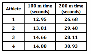
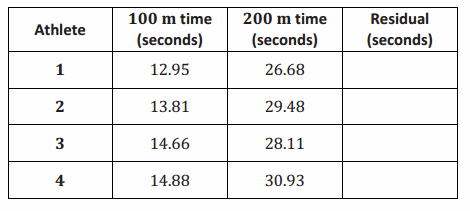
Four athletes on a track team are comparing their personal bests in the 100 meter and 200 meter events. A table of their best times is shown below.
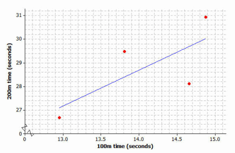
A scatter plot of these results (including the least squares line) is shown below.
Question 1.
Use your calculator or computer to find the equation of the least squares line.
Answer:
y=7.526+1.5115x, where x represents 100-meter time and y represents 200-meter time.
Question 2.
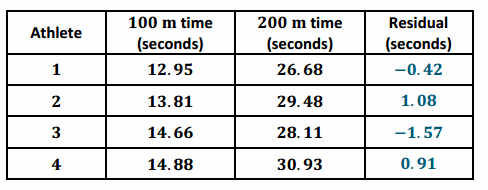
Use your equation to find the predicted 200-meter time for the runner whose 100-meter time is 12.95 seconds. What is the residual for this athlete?
Answer:
y=7.526+1.5115(12.95)≈27.10
Residual =26.68-27.10=-0.42
The predicted 200″ ” m time for the runner is 27.10 seconds. The residual is -0.42 seconds.
Question 3.
Calculate the residuals for the other three athletes. Write all the residuals in the table given below.
Answer:
Question 4.
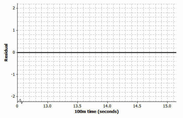
Using the axes provided below, construct a residual plot for this data set.
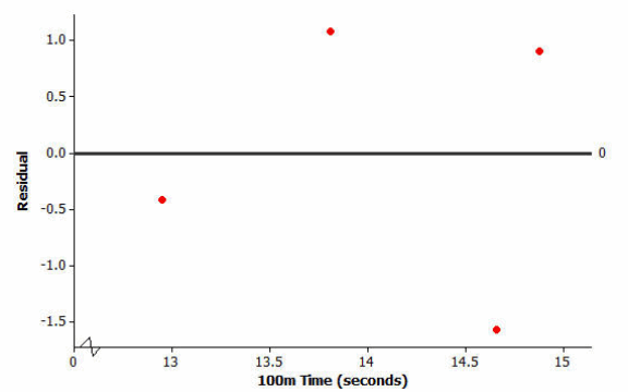
Answer:
Eureka Math Algebra 1 Module 2 Lesson 16 Exit Ticket Answer Key
Question 1.
Suppose you are given a scatter plot (with least squares line) that looks like this:
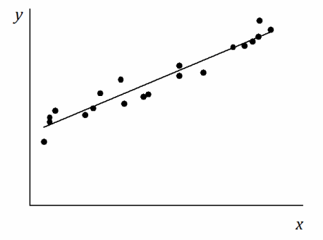
What would the residual plot look like? Make a quick sketch on the axes given below. (There is no need to plot the points exactly.)
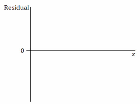
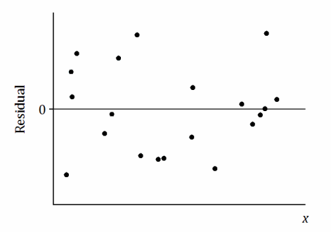
Answer:
Question 2.
Suppose the scatter plot looked like this:
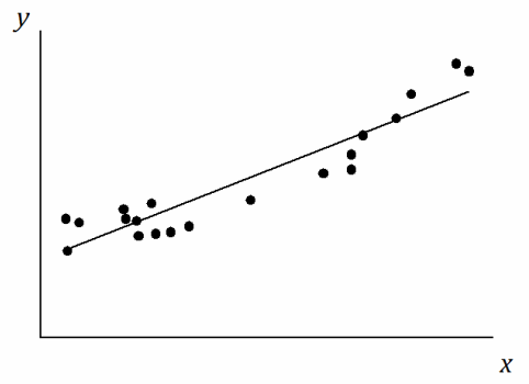
Make a quick sketch on the axes below of how the residual plot would look.
Answer:
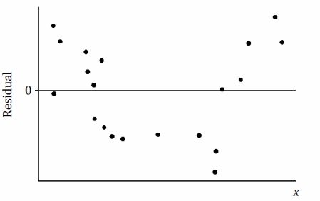
Note: It is important that students begin to see the general shape of the pattern in the residual plot, a random scatter of points in Problem 1, and a U-shape in Problem 2. Beyond that, the details of the residual plots are not of concern at this point in the study of residuals.