Engage NY Eureka Math Algebra 2 Module 4 Lesson 27 Answer Key
Eureka Math Algebra 2 Module 4 Lesson 27 Exercise Answer Key
Exercises 1 – 4: Carrying Out a Randomization Test
The following are the general steps for carrying out a randomization test to analyze the results of an experiment. The steps are also presented in the context of the tomato example of the previous lessons.
Step 1 – Develop competing claims: no difference versus difference.
One claim corresponds to no difference between the two groups in the experiment. This claim is called the null hypothesis.
→ For the tomato example, the null hypothesis is that the nutrient treatment is not effective in increasing tomato weight. This is equivalent to saying that the average weight of treated tomatoes may be the same as the average weight of nontreated (control) tomatoes.
The competing claim corresponds to a difference between the two groups. This claim could take the form of a different from, greater than, or less than a statement. This claim is called the alternative hypothesis.
→ For the tomato example, the alternative hypothesis is that the nutrient treatment is effective in increasing tomato weight. This is equivalent to saying that the average weight of treated tomatoes is greater than the average weight of nontreated (control) tomatoes.
Exercise 1.
Previously, the statistic of interest that you used was the difference between the mean weight of the 5 tomatoes in Group A and the mean weight of the 5 tomatoes in Group B. That difference was called Diff. Diff = \(\overline{\boldsymbol{x}}_{A}\) – \(\overline{\boldsymbol{x}}_{B}\). If the treatment tomatoes are represented by Group A and the control tomatoes are represented by Group B, what type of statistically significant values of Diff would support the claim that the average weight of treated tomatoes is greater than the average weight of nontreated (control) tomatoes: negative values of Diff positive values of Diff or both? Explain.
Answer:
For the tomato example, since the treatment group is Group A, the Diff value of \(\overline{\boldsymbol{x}}_{A}\) – \(\overline{\boldsymbol{x}}_{B}\) is \(\bar{x}_{\text {Treatment }}-\bar{x}_{\text {Control }}\).
Since the alternative claim is supported by \(\overline{\boldsymbol{x}}_{\text {Treatment }}>\overline{\boldsymbol{x}}_{\text {Control }}\) we are seeking statistically significant Diff values that are positive since if \(\overline{\boldsymbol{x}}_{\text {Treatment }}>\overline{\boldsymbol{x}}_{\text {Control }}\) then \(\bar{x}_{\text {Treatment }}-\bar{x}_{\text {Control }}\) > 0. Statistically significant values of Diff that are negative in this case would imply that the treatment made the tomatoes smaller on average.
Note: The answer/information above appears in Step 4 of the randomization test of the student material.Step 2 –
Take measurements from each group, and calculate the value of the Diffstatistic from the experiment.
For the tomato example, first, measure the weights of the 5 tomatoes from the treatment group (Group A); next,
measure the weights of the 5 tomatoes from the control group (Group B); finally, compute Diff = \(\overline{\boldsymbol{x}}_{A}\) – \(\overline{\boldsymbol{x}}_{B}\), which will serve as the result from your experiment.
Exercise 2.
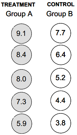
Assume that the following represents the two groups of tomatoes from the actual experiment. Calculate the value of Diff = \(\overline{\boldsymbol{x}}_{A}\) – \(\overline{\boldsymbol{x}}_{B}\). This will serve as the result from your experiment.
These are the same 10 tomatoes used in previous lessons; the identification of which tomatoes are treatment versus control is now revealed.
Answer:
Diff = 7.74 – 5.5 = 2.24
Again, these tomatoes represent the actual result from your experiment. You will now create the randomization distribution by making repeated random assignments of these 10 tomatoes into 2 groups and recording the observed difference in means for each random assignment.
This develops a randomization distribution of the many possible difference values that could occur under the assumption that there is no difference between the mean weights of tomatoes that receive the treatment and tomatoes that don’t receive the treatment.
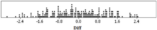
Step 3 – Randomly assign the observations to two groups, and calculate the difference between the group means. Repeat this several times, recording each difference. This will create the randomization distribution for the Diff statistic.
Examples of this technique were presented in a previous lesson. For the tomato example, the randomization distribution has already been presented in a previous lesson and is shown again here. The dots are placed at increments of 0.04 ounces.
For the tomato example, since the treatment group is Group A, the Diff value of \(\overline{\boldsymbol{x}}_{A}\) – \(\overline{\boldsymbol{x}}_{B}\) is \(\overline{\boldsymbol{x}}_{\text {Treatment }}-\overline{\boldsymbol{x}}_{\text {Control }} \text { . }\).
Since the alternative claim is supported by \(\overline{\boldsymbol{x}}_{\text {Treatment }}-\overline{\boldsymbol{x}}_{\text {Control }} \text { . }\), you are seeking statistically significant Diff values that are positive since if \(\overline{\boldsymbol{x}}_{\text {Treatment }}-\overline{\boldsymbol{x}}_{\text {Control }} \text { . }\), then \(\overline{\boldsymbol{x}}_{\text {Treatment }}-\overline{\boldsymbol{x}}_{\text {Control }} \text { . }\) > 0.
Statistically significant values of Diff that are negative, in this case, would imply that the treatment made the tomatoes smaller on average.
Exercise 3.
Using your calculation from Exercise 2, determine the probability of getting a Dill value as extreme as or more
extreme than the Diff value you obtained for this experiment (in Step 2).
Answer:
6 out of 250 is 0.024, which is 2.4%.
Step 5 – Make a conclusion in context based on the probability calculation (Step 4).
If there is a small probability of obtaining a Diff value as extreme as or more extreme than the Diff value you obtained in your experiment, then the Diff value from the experiment is unusual and not typical of chance behavior. Your experiment’s results probably did not happen by chance, and the results probably occurred because of a statistically significant difference in the two groups.
→ In the tomato experiment, 1f you think there is a statistically significant difference in the two groups, you have evidence that the treatment may in fact be yielding heavier tomatoes on average.
If there is not a small probability of obtaining a Diff value as extreme as or more extreme than the Diff value you obtained in your experiment, then your Diff value from the experiment is not considered unusual and could be typical of chance behavior. The experiment’s results may have just happened by chance and not because of a statistically significant difference in the two groups.
→ In the tomato experiment, if you don’t think that there is a statistically significant difference in the two groups, then you do not have evidence that the treatment results in larger tomatoes on average.
In some cases, a specific cutoff value called a significance level might be employed to assist in determining how small this probability must be in order to consider results statistically significant.
Exercise 4.
Based on your probability calculation in Exercise 3, do the data from the tomato experiment support the claim that the treatment yields heavier tomatoes on average? Explain.
Answer:
The a from the tomato experiment support the claim that the treatment yields heavier tomatoes on average. The probability of obtaining a Diff value as extreme as or more extreme than 2.24 is very small if the treatment is ineffective. This means that there is a statistically significant difference between the average weights of the treatment and control tomatoes, with the treatment tomatoes being heavier on average.
Exercises 5 – 10: Developing the Randomization Distribution
Although you are familiar with how a randomization distribution is created in the tomato example, the randomization distribution was provided for you. In this exercise, you will develop two randomization distributions based on the same group of 10 tomatoes.
One distribution will be developed by hand and will contain the results of at least 250 random assignments. The second distribution will be developed using technology and will contain the results of at least 250 random assignments. Once the two distributions have been developed, you will be asked to compare the distributions.
Manually Generated:
Your instructor will provide you with specific guidance regarding how many random assignments you need to carry out. Ultimately, your class should generate at least 250 random assignments, compute the Duff value for each, and record these 250 or more Diff values on a class or an individual dot plot.
Exercise 5.
To begin, write the 10 tomato weights on 10 equally sized slips of paper, one weight on each slip. Place the slips in a container, and shake the container well. Remove 5 slips, and assign those 5 tomatoes as Group A. The remaining tomatoes will serve as Group B.
Answer:
For the manually generated randomization distribution, it states that students can use 10 equally sized pieces of paper to be selected from a container. However, manipulatives such as small chips or checkers would be fine as well.
Exercise 6.
Calculate the mean weight for Group A and the mean weight for Group B. Then, calculate Duff = 8 for this random assignment.
Answer:
See above.
Exercise 7.
Record your Diff value, and add this value to the dot plot. Repeat as needed per your instructor’s request until a manually generated randomization distribution of at least 250 differences has been achieved.
(Note: This distribution will most likely be slightly different from the tomato randomization distribution given earlier in this lesson.)
Answer:
Students’ work will vary. Overall, the manually generated distribution for the Diff statistic in this tomato example should not differ too much from the distribution presented previously in this and other lessons.
Computer Generated
At this stage, you will be encouraged to use a Web-based randomization testing applet/calculator to perform the steps above. The applet is located at http://www.rossmanchance.com/applets/AnovaShuffle.htm. To supplement the instructions below, a screenshot of the applet appears as the final page of this lesson.
Upon reaching the applet, do the following:
→ Press the Clear button to clear the data under Sample Data.
→ Enter the tomato data exactly as shown below. When finished, press the Use Data button.
| Group | Ounces |
| Treatment | 9.1 |
| Treatment | 8.4 |
| Treatment | 8 |
| Control | 7.7 |
| Treatment | 7.3 |
| Control | 6.4 |
| Treatment | 5.9 |
| Control | 5.2 |
| Control | 4.4 |
| Control | 3.8 |
Once the data are entered, notice that dot plots of the two groups appear. Also, the statistic window below the data now says “difference In means” and an Observed Diff value of 2.24 is computed for the experiment’s data (just as you computed in Exercise 2).
By design, the applet will determine the difference of means based on the first group name it encounters in the data set – specifically, it will use the first group name it encounters as the first value in the difference of means calculation. In other words, to compute the difference in means as \(\bar{x}_{\text {Treatment }}-\bar{x}_{\text {Control }}\), a Treatment observation needs to appear prior to any Control observations in the data set as entered.
→ Select the check box next to Show Shuffle Options, and a dot plot template will appear.
→ Enter 250 in the box next to Number of Shuffles, and press the Shuffle Responses button. A randomization distribution based on 250 randomizations (in the form of a histogram) is created.
This distribution will most likely be slightly different from both the tomato randomization distribution that appeared earlier in this lesson and the randomization distribution that was manually generated in Exercise 7.
Exercise 8.
Write a few comments comparing the manually generated distribution and the computer-generated distribution. Specifically, did they appear to have roughly the same shape, center, and spread?
Answer:
Students should compare and contrast the shape, center, and spread characteristics of the manually generated and computer-generated distributions. There should be a great deal of similarity, but outliers and slightly different clustering patterns may be present.
The applet also allows you to compute probabilities. For this case:
→ Under Count Samples, select Greater Than. Then, in the box next to Greater than, enter 2.2399. Since the applet computes the count value as strictly greater than and not greater than or equal to, in order to obtain the probability of obtaining a value as extreme as or more extreme than the Observed Diff value of 2.24, you will need to enter a value just slightly below 2.24 to ensure that Diff observations of 2.24 are included in the count.
→ Select the Count button. The probability of obtaining a Diff value of 2.24 or more in this distribution will be computed for you.
The applet displays the randomization distribution in the form of a histogram, and it shades in red oil histogram classes that contain any difference values that meet your Count Samples criteria. Due to the grouping and binning of the classes, some of the red shaded classes (bars) may also contain difference values that do not fit your Count Samples criteria. Just keep in mind that the Count value stated in red below the histogram will be exact; the red shading in the histogram may be approximate.
Exercise 9.
How did the probability of obtaining a Diff value of 2.24 or more using your computer-generated distribution compare with the probability of obtaining a Diff value of 2.24 or more using your manually generated distribution?
Answer:
It is expected that the event of finding a Diff value of 2.24 or more will have a similarly rare probability of occurrence in both the manually generated and the computer-generated distributions.
Exercise 10.
Would you come to the same conclusion regarding the experiment using either the computer-generated or manually generated distribution? Explain. Is this the same conclusion you came to using the distribution shown earlier in this lesson back in Step 3?
Answer:
Based on the assumptions regarding the similarity of the distributions as described in Exercise 9 above, it is expected that students will come to the same conclusion (that the treatment is effective) from both the manually generated and the computer-generated distributions as was seen in Exercise 4.
Eureka Math Algebra 2 Module 4 Lesson 27 Problem Set Answer Key
Question 1.
Using the 20 observations that appear in the table below for the changes in pain scores of 20 individuals, use the anova Shuffle applet to develop a randomization distribution of the value Diff = \(\overline{\boldsymbol{x}}_{A}\) – \(\overline{\boldsymbol{x}}_{B}\) based on 100 random assignments of these 20 observations into two groups of 10. Enter the data exactly as shown below. Describe similarities and differences between this new randomization distribution and the distribution shown.
Answer:
Answers will vary, but the distribution should not differ too much from the distribution presented previously in this lesson (Exit Ticket Problem 3) and other lessons.
Question 2.
In a previous lesson, the burn times of 6 candles were presented. It is believed that candles from Group A will burn longer on average than candles from Group B. The data from the experiment (now shown with group identifiers) are provided below.
| Group | Burntime |
| A | 18 |
| A | 12 |
| B | 9 |
| A | 6 |
| B | 3 |
| B | 0 |
Perform a randomization test of this claim. Carry out all 5 steps, and use the Anova Shuffle applet to perform Steps 2 – 4. Enter the data exactly as presented above, and in Step 3, develop the randomization distribution based on 200 random assignments.
Answer:
Step 1 – Null hypothesis: Candles from Group A will burn for the same amount of time on average as candles from Group B (no difference in average burn time).
Alternative hypothesis: Candles from Group A will burn longer on average than candles from Group B.
Step 2 – Diff = 12 – 4 = 8
Step 3 – Randomization distribution of Diff developed by the student
Step 4 – Compute the probability of Diff greater than or equal to 8 (value should be close to 10%).
Step 5 – While there are no specific criteria stated in the question for what is a “small probability,” students should consider probability values from previous work in determining “small” versus “not small” Again, student values will vary. The important point is that students’ conclusions should be consistent with the probability value and students’ assessment of that value as follows:
If students deem the probability to be “small,” then they should state a conclusion based on a statistically significant result. More specifically, due to the small chance of obtaining a Diff value os extreme as or more extreme than the Diff value obtained in the experiment, it is believed that the observed difference did not happen by chance alone, and we support the claim that the Group A candles burn longer on average.
If students deem the probability to be NOT “small,” then they should state a conclusion based on a result that is NOT statistically significant. More specifically, it is believed that the observed difference may have occurred by chance, and we do NOT have evidence to support the aim that the Group A candles burn longer on average.
Eureka Math Algebra 2 Module 4 Lesson 27 Exit Ticket Answer Key
In the Exit Ticket of a previous lesson, an experiment with 20 subjects investigating a new pain reliever was introduced. The subjects were asked to communicate their level of pain on a scale of 0 to 10 where 0 means no pain and 10 means worst pain. Due to the structure of the scale, a patient would desire a lower value on this scale after treatment for pain.
The value “Change in Score” was recorded as the subject’s pain score after treatment minus the subject’s pain score before treatment. Since the expectation is that the treatment would lower a patient’s pain score, a negative value would be desired for ‘thangeinScore.” For example, a “ChangeinScore” value of -2 would mean that the patient was in less pain (for example, now at a 6, formerly at an 8).
In the experiment, the null hypothesis would be that the treatment had no effect. The average change in pain score for the treatment group would be the same as the average change in pain score for the placebo (control) group.
Question 1.
The alternative hypothesis would be that the treatment was effective. Using this context, which mathematical relationship below would match this alternative hypothesis? Choose one.
a. The average change in pain score (the average “ChangeinScore”) for the treatment group would be less than the average change in pain score for the placebo group (supported by \(\overline{\boldsymbol{x}}_{\text {Treatment }}<\overline{\boldsymbol{x}}_{\text {Control }}\) or \(\overline{\boldsymbol{x}}_{\text {Treatment }}-\overline{\boldsymbol{x}}_{\text {Control }}\) < 0).
b. The average change in pain score (the average “ChangeinScore”) for the treatment group would be greater than the average change in pain score for the placebo group (supported by \(\overline{\boldsymbol{x}}_{\text {Treatment }}>\overline{\boldsymbol{x}}_{\text {Control }}\), or \(\overline{\boldsymbol{x}}_{\text {Treatment }}-\overline{\boldsymbol{x}}_{\text {Control }}\) > 0).
Answer:
Choice (a): The average change in pain score (the average “ChangeinScore “) for the treatment group would be less than the average change in pain score for the placebo group.
Question 2.
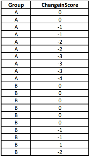
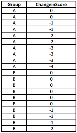
Imagine that the 20 “ChangeinScore” observations below represent the change in pain levels of the 20 subjects (chronic pain sufferers) who participated in the clinical experiment. The 10 individuals in Group A (the treatment group) received a new medicine for their pain while the 10 individuals in Group B received the pill with no medicine
placebo). Assume for now that the 20 individuals have similar initial pain levels and medical conditions. Calculate
the value of Diff = \(\overline{\boldsymbol{x}}_{A}\) – \(\overline{\boldsymbol{x}}_{B}\) = \(\overline{\boldsymbol{x}}_{\text {Treatment }}-\overline{\boldsymbol{x}}_{\text {Control }} \text { . }\). This is the result from the experiment.
Answer:
Diff = -1.4 (Group A mean= -1.9; Group B mean= -0.5)
Question 3.
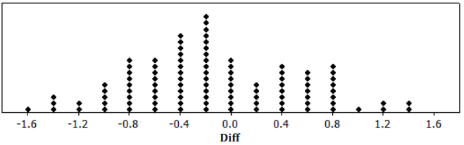
Below is a randomization distribution of the value Diff = \(\overline{\boldsymbol{x}}_{A}\) – \(\overline{\boldsymbol{x}}_{B}\) based on 100 random assignments of these 20 observations into two groups of 10 (shown in a previous lesson).
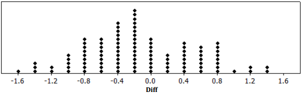
With reference to the randomization distribution above and the inequality in your alternative hypothesis, compute the probability of getting a Diff value as extreme as or more extreme than the Diff value you obtained in the experiment.
Answer:
4% (4 out of 100).
Question 4.
Based on your probability value from Problem 3 and the randomization distribution above, choose one of the following conclusions:
a. Due to the small chance of obtaining a Diff value as extreme as or more extreme than the Diff value obtained in the experiment, we believe that the observed difference did not happen by chance alone, and we support the claim that the treatment is effective.
b. Because the chance of obtaining a Diff value as extreme as or more extreme than the Diff value obtained in the experiment is not small, it is possible that the observed difference may have happened by chance alone, and we cannot support the claim that the treatment is effective.
Answer:
Choice (a): Due to the small chance of obtaining a Diff value as extreme as or more extreme than the Diff value obtained in the experiment, we believe that the observed difference did not happen by chance alone, and we support the claim that the treatment is effective.