Engage NY Eureka Math Algebra 2 Module 4 Lesson 9 Answer Key
Eureka Math Algebra 2 Module 4 Lesson 9 Example Answer Key
Example 1: Heights of Dinosaurs and the Normal Curve
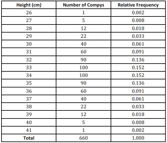
A paleontologist studies prehistoric life and sometimes works with dinosaur fossils. The table below shows the distribution of heights (rounded to the nearest inch) of 660 procompsognathids, otherwise known as compys.
The heights were determined by studying the fossil remains of the compys.
Exercises 1 – 8:
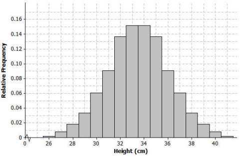
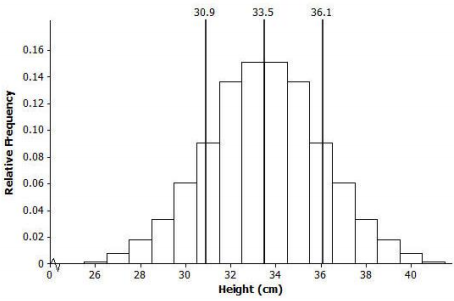
The following is a relative frequency histogram of the compy heights:
Exercise 1.
What does the relative frequency of 0.136 mean for the height of 32 cm?
Answer:
13.6% of the 660 compys were 32 cm tall.
Exercise 2.
What is the width of each bar? What does the height of the bar represent?
Answer:
Each bar has a width of 1 cm. The height of the bar is the relative frequency for the corresponding compy height.
Exercise 3.
What is the area of the bar that represents the relative frequency for compys with a height of 32 cm?
Answer:
The area of the bar is equal to the relative frequency of 0.136.
Exercise 4.
The mean of the distribution of compy heights is 33.5 cm, and the standard deviation is 2.56 cm. Interpret the mean and standard deviation in this context.
Answer:
- The mean of 33.5 cm is the average height of the compys in the sample. It can be interpreted as a typical compy height.
- The standard deviation of 2.56 cm is the typical distance that a campy height is from the mean height.
Exercise 5.
Mark the mean on the graph, and mark one deviation above and below the mean.
a. Approximately what percent of the values in this data set are within one standard deviation of the mean (i.e., between 33.5 cm – 2.56 cm = 30.94 cm and 33.5 cm + 2.56 cm = 36.06 cm)?
Answer:
0.091 + 0.136 + 0.152 + 0.152 + 0.136 +0.091 = 0.758 = 75.8%
b. Approximately what percent of the values in this data set are within two standard deviations of the mean?
Answer:
Between 29 and 38, about 94%
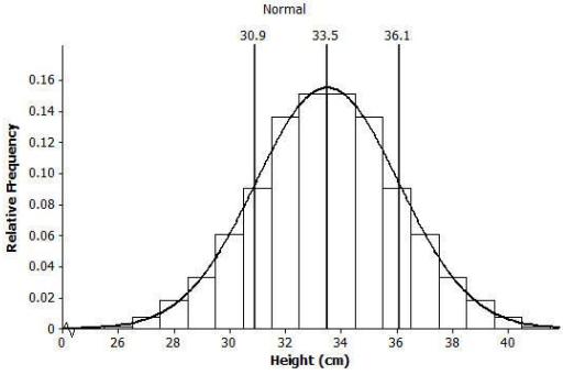
Exercise 6.
Draw a smooth curve that comes reasonably close to passing through the midpoints of the tops of the bars in the histogram. Describe the shape of the distribution.
Answer:
The curve is bell-shaped and approximately symmetric and mound-shaped.
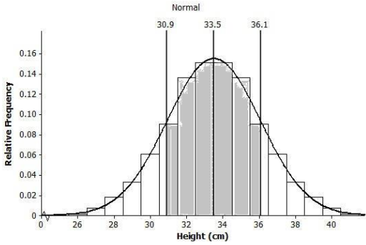
Exercise 7.
Shade the area of the histogram that represents the proportion of heights that are within one standard deviation of the mean.
Answer:
Exercise 8.
Based on our analysis, how would you answer the question, “How tall was a compy?”
Answer:
Answers will vary. It is likely that students will say the height was between 31 cm and 36 cm.
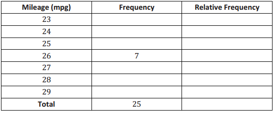
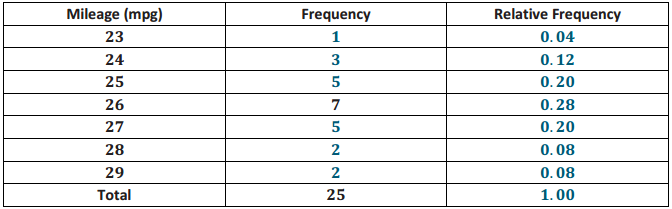
Example 2: Gas Mileage and the Normal Distribution
A normal curve is a smooth curve that is symmetric and bell shaped. Data distributions that are mound shaped are often modeled using a normal curve, and we say that such a distribution is approximately normal. One example of a distribution that is approximately no4mal is the distribution of compy heights from Example t. Distributions that are approximately normal occur in many different settings. For example, a salesman kept track of the gas mileage for his car over a 25-week span.
The mileages (miles per gallon rounded to the nearest whole number) were
23, 27, 27, 28, 25, 26, 25, 29, 26, 27, 24, 26, 26, 24, 27, 25, 28, 25, 26, 25, 29, 26, 27, 24, 26.
Exercise 9:
Exercise 9.
Consider the following:
a. Use technology to find the mean and standard deviation of the mileage data. How did you use technology to assist you?
Answer:
Mean = 26.04 mpg
Standard deviation = 1.54 mpg
The graphing calculator does several tedious calculations for me. I entered the data into lists and was able to indicate what calculations. I wanted done by writing an expression using lists. I did not have to set up the organization to find the standard deviation and perform the rather messy calculations.
b. Calculate the relative frequency of each of the mileage values. For example, the mileage of 26 mpg has a frequency of 7. To find the relative frequency, divide 7 by 25. the total number of mileages recorded. Complete the following table:
Answer:
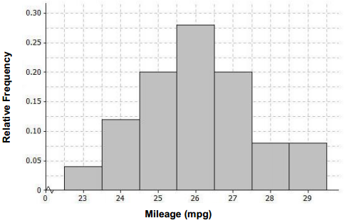
c. Construct a relative frequency histogram using the scale below.
Answer:
Completed histogram:
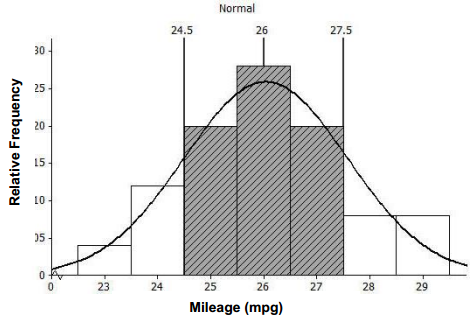
d. Describe the shape of the mileage distribution. Draw a smooth curve that comes reasonably close to passing through the midpoints of the tops of the bars in the histogram. Is this approximately a normal curve?
Answer:
The shape is approximately normal See the graph in part (e).
e. Mark the mean on the histogram. Mark one standard deviation to the left and right of the mean. Shade the area of the histogram that represents the proportion of mileages that are within one standard deviation of the mean. Find the proportion of the data within one standard deviation of the mean.
Answer:
One standard deviation to the left (or below) the mean: 26.04 – 1. 54 = 24.5
One standard deviation to the right (or above) the mean: 26.04 + 1.54 = 27.58
The proportion of the data within one standard deviation of the mean is approximately 0.68 (which is the sum of 0.20 + 0.28 + 0.20).
Eureka Math Algebra 2 Module 4 Lesson 9 Problem Set Answer Key
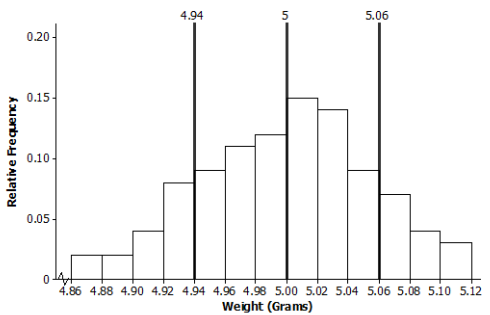
Question 1.
Periodically the U.S. Mint checks the weight of newly minted nickels. Below is a histogram of the weights (In grams) of a random sample of loo new nickels.
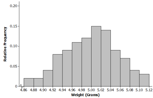
a. The mean and standard deviation of the distribution of nickel weights are 5.00 grams and 0. 06 gram, respectively. Mark the mean on the histogram. Mark one standard deviation above the mean and one standard deviation below the mean.
Answer:
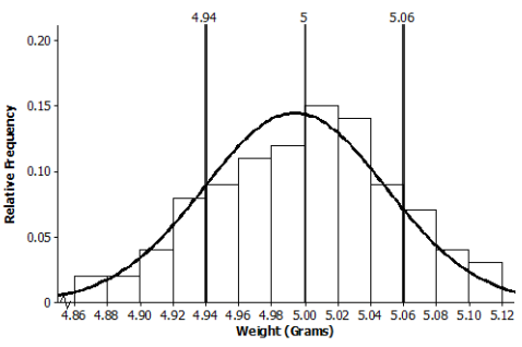
b. Describe the shape of the distribution. Draw a smooth curve that comes reasonably close to passing through the midpoints of the tops of the bars in the histogram. Is this approximately a normal curve?
Answer:
The shape is approximately normal.
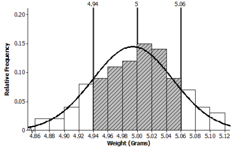
c. Shade the area of the histogram that represents the proportion of weights within one standard deviation of the mean. Find the proportion of the data within one standard deviation of the mean.
Answer:
0.09 + 0.11 + 0.12 + 0.15 + 0.14 + 0.09 = 0.70
Question 2.
Below is a relative frequency histogram of the gross (in millions of dollars) for the all-time top-grossing American movies (as of the end of 2012). Gross is the total amount of money made before subtracting out expenses, like advertising costs and actors’ salaries.
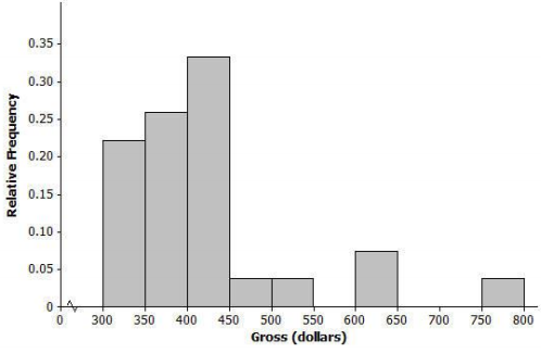
a. Describe the shape of the distribution of all-time top-grossing movies. Would a normal curve be the best curve to model this distribution? Explain your answer.
Answer:
The shape is skewed to the right. A normal curve would not be the best curve to model the distribution.
b. Which of the following is a reasonable estimate for the mean of the distribution? Explain your choice.
i. 325 million
ii. 375 million
iii. 425 million
Answer:
(iii) 425 million is a reasonable estimate since this is a skewed distribution, and the mean will be pulled toward the outliers.
c. Which of the following is a reasonable estimate for the sample standard deviation? Explain your choice.
i. 50 million
ii. 100 million
iii. 200 million
Answer:
(ii) 100 million is a reasonable estimate because 50 million is too small, and 200 million is too large to be considered a typical deviation from the mean.
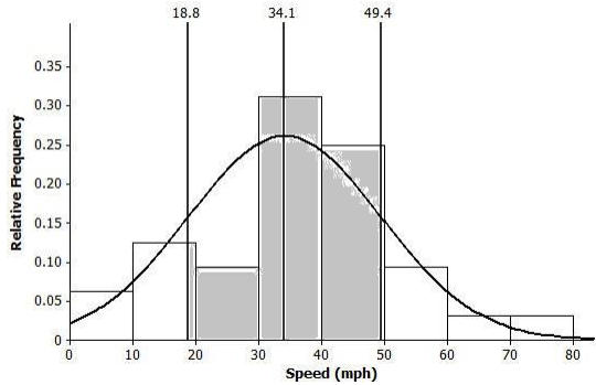
Question 3.
Below is a histogram of the top speed of different types of animals.
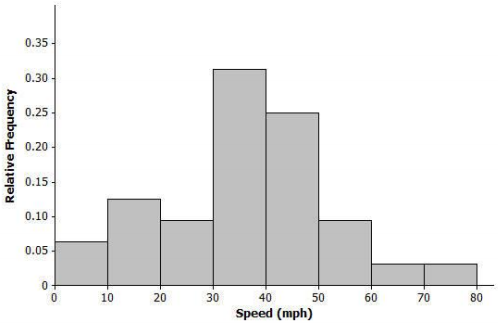
a. Describe the shape of the top speed distribution.
Answer:
Approximately normal
b. Estimate the mean and standard deviation of this distribution. Describe how you made your estimate.
Answer:
Mean is approximately 40 mph, and standard deviation is about 15 mph. Answers will vary in terms of how the estimate was made.
Note: Students could roughly estimate the mean by locating a balance point of the distribution. The standard deviation could be estimated by a typical deviation from the mean that was developed in Lesson 8.
c. Draw a smooth curve that is approximately a normal curve. The actual mean and standard deviation of this data set is 34.1 mph and 15.3 mph, respectively. Shade the area of the histogram that represents the proportion of speeds that are within one standard deviation of the mean.
Answer:
Eureka Math Algebra 2 Module 4 Lesson 9 Exit Ticket Answer Key
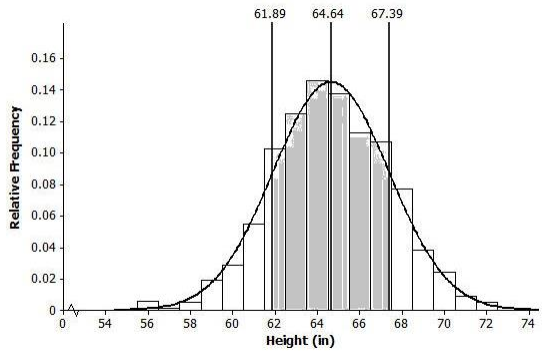
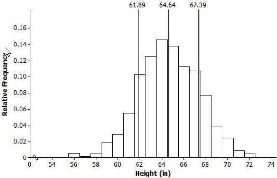
The histogram below shows the distribution of heights (to the nearest inch) of 1,000 young women.
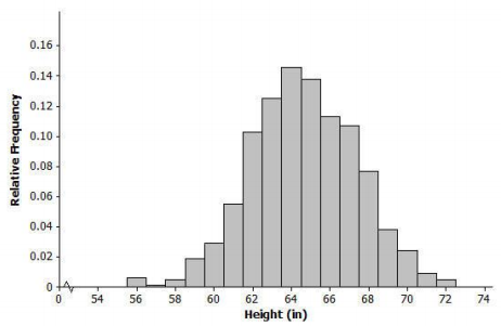
Question 1.
What does the width of each bar represent? What does the height of each bar represent?
Answer:
Each bar represents a 1-inch range of heights. For example, the bar above 56 represents heights between 55.50 and 56.49 inches. The height of each bar represents the proportion of the 1,000 women in that 1-inch height range.
Question 2.
The mean of the distribution of women’s heights is 64. 6 in., and the standard deviation is 2.75 in. Interpret the mean and standard deviation in this context.
Answer:
The mean is the average height of the 1,000 women, and it can be interpreted as a typical height value. The standard deviation is the typical number of inches that a woman’s height is from the mean.
Question 3.
Mark the mean on the graph, and mark one deviation above and below the mean. Approximately what proportion of the values in this data set are within one standard deviation of the mean?
Answer:
0.10 + 0.12 + 0.14 + 0.13 + 0.11 + 0.105 = 0.705 ≈ 0.71
Question 4.
Draw a smooth curve that comes reasonably close to passing through the midpoints of the tops of the bars in the histogram. Describe the shape of the distribution.
Answer:
Approximately normal (bell shaped and approximately symmetric)
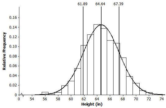
Question 5.
Shade the area of the histogram that represents the proportion of heights that are within one standard deviation of the mean.
Answer: